Non-Differentiable Functions in Machine Learning

Here is one of the rare generally applicable statements in machine learning: letting the family of functions implemented by a model reflect true knowledge about the data will make the model much better. The model will search over a smaller parameter space, with a better chance of generalizing well, and a dramatically reduced need for data and computational expense. In that context, non-differentiable functions like $\mathrm{max}(x)$, $\mathrm{abs}(x)$ or $\mathrm{sgn}(x)$ are a useful tool because they can express break points, transitions, and so on. Alternatively, you may be using a deep learning framework to solve constrained optimization problems, which might be done by using non-differentiable step functions in the objective function. It’s worth thinking through what it might mean to use these types of functions as part of a model.

First, in the context of neural networks, some non-differentiable functions are surprisingly benign. This is evidenced by the prevalence of the non-differentiable ReLU as activation function. On the face of it, this might seem surprising because these networks are trained with gradient descent, but with random initilialization the chance of evaluating the network exactly at the point of discontinuous derivative is effectively zero, and even then, deep learning frameworks like pytorch can often automatically handle non-differentiability using subgradients. A more significant issue is that non-differentiable functions can result in unpleasant loss landscapes. This is again mostly an issue when you are fitting small models, where you are more likely to be invested in converging to a specific minimum, for example because the parameter values have precise, interpretable meaning. The large deep learning models that fall into the overparametrized paradigm are not conducive to this, and their flattened loss functions with many minima are considered a feature and not a bug.

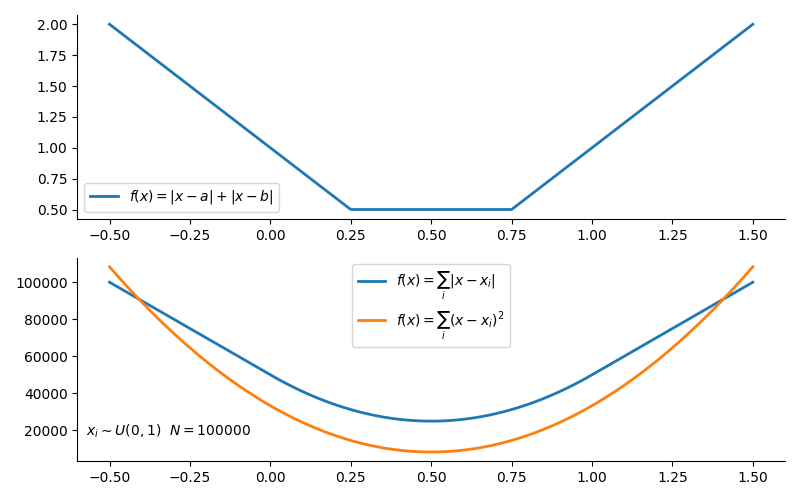
An potentially troublesome example example for that comes up with small models is L1 (absolute error) loss, which is useful for its robustness but doesn’t have a unique solution like L2 (squared error) loss. To illustrate, consider $f(x) = |x-a| + |x-b|$, which is $L1$ loss for two datapoints in one dimension. The expression doesn’t have a unique minimum, but is minimal over a contiguous subset $x_{min} \in [a,b]$. Minimizing this using a standard gradient descent framework can give different values of $x$ with each training. A larger number of points makes perfect flatness unlikely, but compared to e.g. the least square differences, the curvature near the minimum flatter and give less stable results. As usual, the 1D example is generous: in higher dimensions intuition fails fast. In practice it won’t be clear if convergence problems have to do with the model or whether the data is just too noisy.

Top: 1-Dimensional L1 loss for two points $a=0.25$ and $b=0.75$. Bottom: 1-Dimensional L1 (absolute value) and L2 (least squares) loss for a large number of points sampled from a uniform distribution $x_i\sim\mathbb{U}(0,1)$.

Optimization problems involving weird functions is the bread and butter of the (convex) optimization specialists, and to take matters seriously, there is no way around e.g. (Boyd & Vandenberghe, 2004), for which there are also excellent lectures online (70% math, 30% Boyd jokes!). Considerable work is going into this in machine learning as well, both in terms of theory and in terms of implementation (a google search leads down more than one rabbit hole). The topic of non-differentiable functions in machine learning also goes deep in the sense that many settings aren’t conducive to straight-forward optimization with gradient descent (things like reinforcement learning, GANs, probabilistic models fit with MCMC, non-convex optimization tackled with techniques like genetic algorithms and so on and on – getting to use gradient methods is a win in and off of itself).

The point of this post is to sidestep all those deeper discussions. The non-differentiable functions that come up in practice often have smooth approximations that can be gradually sharpened to approach the exact case. An approximate model will usually be equivalent to the exact case for the purpose of fitting data, and it is possible to build intuition by observing the behavior of the model as the discontinuity is removed and replaced. In a case like the introductory example with $L1$ (absolute value) loss, the approximation can re-introduce a little bit of curvative into the loss function that stabilizes the model. As a considerable bonus, removing the non-differentiable point allows for the use of efficient second-order optimization methods like Newton’s method (some software handles this even so, but that is another story).

Below are some approximations of common non-differentiable elements, roughly in the order in which I find them useful. Approximations, in general, are not unique, and other functions can be found that may be more suitable.

It should also be noted that there is a relatively general approach to producing smooth approximations, which is to use mollifiers (though I’ve never actually heard the term “mollifier” used in anger). The basic idea is that the convolution of a function with a dirac delta function gives you back that original function (think: identity operation), and the convolution of a function with a smooth approximation to the dirac delta function gives you back a smooth approximation to that function. On $\mathbb{R}^n$, convolution involves integration. The usual, but not the only, way to approximate a dirac delta function is a Gaussian with variance approaching zero (also listed below). So, if you need something custom built, and finding the convolution of your function with, for example, a Gaussian sounds like a good idea, then this is a great way to go.

The Heaviside Step Function, $\Theta(x-a)$, with Sigmoids

This is the building block for building any piecewise continuous function.

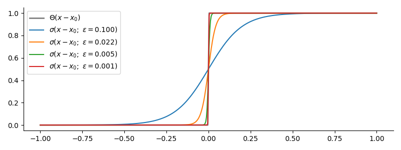
$$ \begin{equation} \Theta\left(x-x_0\right) = \left\{\begin{array}{ll} 0 & \text{for } x < x_0\\ 0.5 & \text{if } x = x_0\\ 1 & \text{for } x > x_0 \end{array}\right. \end{equation} $$

The step function isn’t always defined to have $\Theta(0) = 0.5$ at the break point “$x_0$”, but that normally won’t make a difference when fitting to fuzzy data. The common way to approximate the step function is to use any kind of sigmoid, including the most famous sigmoid, the logistic function.

$$ \sigma\left(x-x_0; \epsilon\right) = \frac{1}{1+e^{-\frac{\left(x-x_0\right)}{\epsilon}}} $$

Physicists will recognize this function as the Fermi-Dirac distribution, only that the $x$-axis is flipped. The breakpoint $x_0$ corresponds to the Fermi Energy, and $\epsilon$ is the Boltzman-scaled temperature $kT$. When $\epsilon$, or, if you wish, the temperature, is zero, the approximation becomes exact.

Heaviside step function $\Theta(x-x_0)$ and approximation with a logistic function $\sigma(x-x_0;\epsilon)$ for $x_0=0$ and different values of $\epsilon$

Step functions are enough to build a lot of useful things. For example:

Top-Hat Function or Square Well, $T(x-x_0;a,b)$

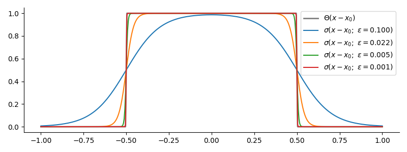
$$ \begin{equation} T\left(x-x_0; a,b\right) = \left\{\begin{array}{ll} 0 & \text{for } x < a;\ x > b\\ 0.5 & \text{if } x \in \{a,b\}\\ 1 & \text{for } a < x < b \end{array}\right. \end{equation} $$

For the sake of one example of how step functions can be used to build useful piecewise linear things, a top hat function can be built with two step functions as $T\left(x-x_0; a,b\right) = \Theta(x-a) - \Theta(x-b)$. By flipping the sign, you can make a square well for your loss function that allows you to effectively perform constrained optimization without unveiling e.g. convex optimization code.

Tophat function $T(x;a,b)$ with boundaries $a=-0.5$ and $b=0.5$, and approximations using logistic functions $\sigma(x-a;\epsilon) - \sigma(x-b;\epsilon)$ for different values of $\epsilon$

Rectifier or ReLu, $\mathrm{max}(x_0,x)$ with $\mathrm{SoftPlus}$

This function is famous because it is used in neural networks and, indeed, is normally replaced by a smooth approximation because it was giving people trouble.

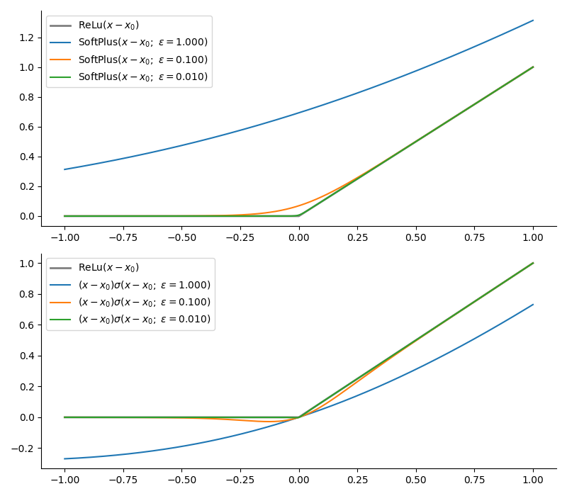
$$ \begin{equation} \mathrm{ReLu}\left(x-x_0\right) = \mathrm{max}(x_0,x)= \left\{\begin{array}{ll} 0 & \text{for } x < x_0\\ x & \text{for } x > x_0 \end{array}\right. \end{equation} $$

The canonical way to remedy the discontinuity is the $\mathrm{Softplus}$ function, which has form:

$$ \mathrm{Softplus}(x-x_0;\epsilon) = \epsilon\mathrm{ln}\left(1+e^{ \frac{x-x_0}{\epsilon}}\right) $$

But you can also build it with a step function as $\mathrm{ReLu}\left(x-x_0\right) = \left(x_0-x\right)\Theta\left(x_0-x\right)$ and use sigmoids. The two approximations approach the exact case from “above” and “below” respectively.

ReLu function $\mathrm{ReLu}(x-x_0)$ with $x_0=0$, and approximations using $\mathrm{Softplus}(x-x_0;\epsilon)$ and using a logistic function $(x-x_0)\sigma(x-x_0;\epsilon)$ for different values of $\epsilon$.

Vector Minimum, Maximum and Vector Dimension with $\mathrm{SoftMax}$

The $\mathrm{SoftMax}$ function will be familiar as the output layer of neural networks used for classification problems. This is because it happens to map from $\mathbb{R}^N$ to a Dirichlet distribution, which is how you would describe the probability distribution of an $N$-way categorical event: the output of the $\mathrm{SoftMax}$ is an $N$-dimensional vector $\mathbf{y} = \mathrm{SoftMax}(x)$ with the properties that $y_i\in[0,1]$ for all $y_i\in\mathbf{y}$ and $||\mathbf{y}||_1 = \sum_i y_i = 1$. The in-built exponential mapping also has the perk that it ought to induce deeper layers to deal in activations on the order of log-probabilities, which is numerically wise. Let $\mathbf{x}$ be an $N$-dimensinal vector, then the $i$th output of $\mathrm{SoftMax}$ is normally expressed as:

$$ \begin{equation} \mathrm{SoftMax}\left(\mathbf{x}\right)_i = \frac{e^{x_i}}{\sum_j^N e^{x_j}} \end{equation} $$

I say “normally” because there are numerical issues with using this formulation to do with the exponential functions that can be avoided using a trick. Using i.e. a PyTorch inbuilt function ought to take that into account. Introducing a parameter $\epsilon$:

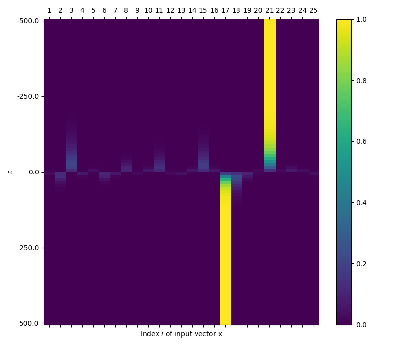
$$ \begin{equation} \mathrm{SoftMax}\left(\mathbf{x};\epsilon\right)_i = \frac{e^{\epsilon x_i}}{\sum_j^N e^{\epsilon x_j}} \end{equation} $$

Three interesting limits emerge:

$$ \begin{equation} \begin{array}{l} \lim_{\epsilon\rightarrow0}\mathrm{SoftMax}\left(\epsilon\mathbf{x}\right)_i = \frac{1}{N}\\ \lim_{\epsilon\rightarrow\infty}\mathrm{SoftMax}\left(\epsilon\mathbf{x}\right)_i = \delta\left(x_i - \mathrm{max}(\mathbf{x})\right)\\ \lim_{\epsilon\rightarrow-\infty}\mathrm{SoftMax}\left(\epsilon\mathbf{x}\right)_i = \delta\left(x_i - \mathrm{min}(\mathbf{x})\right)\\ \end{array} \end{equation} $$

At $\epsilon\rightarrow0$, the function simply returns the inverse of the vector dimension. For large negative and positive $\epsilon$, you get one-hot encoded vector that is $1$ at the location of the minimum and maximum respectively and $0$ elsewhere.

SoftMax function of some $N$-dimensional input vector $\mathbf{x}$ for different values of $\epsilon$. For $\epsilon=0$, all entries are mapped to the same value of $1/N$. For intermediate values, larger values are amplified and smaller values suppressed. For large $\epsilon$, the entry corresponding to the largest vector element is $1$ and all others are $0$.

Minimum and Maximum Values, $\mathbf{min}(\mathbf{x})$ & $\mathbf{max}(\mathbf{x})$

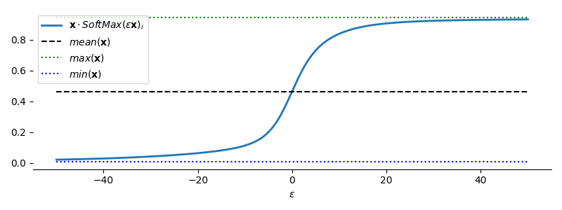
The one-hot encoding of the minimum and maximum can be used to pick out the actual value from a vector by taking the dot product. The result is tunable continuously and gives back the mean value for $\epsilon=0$ (though there are nicer ways to generate the mean!):

$$ \begin{equation} \begin{array}{l} \lim_{\epsilon\rightarrow0}\mathbf{x}\cdot\mathrm{SoftMax}\left(\epsilon\mathbf{x}\right)_i = \mathrm{mean}(\mathbf{x})\\ \lim_{\epsilon\rightarrow\infty}\mathbf{x}\cdot\mathrm{SoftMax}\left(\epsilon\mathbf{x}\right)_i = \mathrm{max}(\mathbf{x})\\ \lim_{\epsilon\rightarrow-\infty}\mathbf{x}\cdot\mathrm{SoftMax}\left(\epsilon\mathbf{x}\right)_i = \mathrm{min}(\mathbf{x})\\ \end{array} \end{equation} $$

Result of $\mathbf{x}\cdot\mathrm{SoftMax}(\epsilon\mathbf{x})$ for different values of $\epsilon$. The function lets you tune between $\mathrm{min}(\mathbf{x})$ to $\mathrm{max}(\mathbf{x})$, passing through $\mathrm{mean}(\mathbf{x})$ at $\epsilon=0$. Here $\mathbf{x}\in\mathbb{R}^{100}$ and was generated from a uniform distribution $\mathbf{x}\sim\mathbb{U}(0,1)$.

If-Elif-Else

The softmax can also be used to build if-elif-else conditionals. The if/elif statements require a set of functions $f_i(x)$ and a constant $c$ so that if condition $i$ is met, $f_i(x) > f_j(x)$ for all $j\neq i$ and $f_i(x) > c$, and $f_i(x) < c$ if condition $i$ is not met. The functions $f_i(x)$ themselves also need to be differentiable. You can often also build these conditionals by using step functions.

Top-K Error

Until I find time to write this out, see this paper. It’s more elegant than what I came up with.

Dirac Delta Function, $\delta(x-x_0)$, with a Gaussian

The Dirac Delta function is often described as a function that has a single infinite spike at the origin, but that simplicity is slightly misleading, because is it not a function in traditional sense and behaves a little differently. It is defined meaningfully only in the context of integration:

$$ \begin{equation} \int_A f(x)\delta(x-x_0) dx = f(x_0) \end{equation} $$

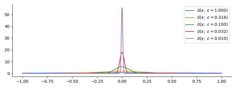
Where $x_0\in A$. Because of this you are probably only going to encounter it in the context of doing analytical calculations, because trying to handle infinitely thin, infinitely sharp spikes numerically is a bad idea. As mentioned at the outset, a smooth approximation to the Dirac Delta function can be used to create a smooth approximation to a function by calculating the convolution with it. The most common, but not the only, way to create a smooth approximation to the Dirac Delta function is:

$$ \begin{equation} \delta_\epsilon(x) = \frac{1}{|\epsilon|\sqrt{\pi}}e^{-\left(\frac{x}{\epsilon}\right)^2} \end{equation} $$

To create a smooth approximation to a function $f(x)$, calculate:

$$ \begin{equation} f_\epsilon(x) = \int f(x')\delta_\epsilon(x'-x) dx' \end{equation} $$

Smooth approximation to a dirac delta function using a Gaussian $\delta_\epsilon(x) = \frac{1}{|\epsilon|\sqrt{\pi}}e^{-\left(\frac{x}{\epsilon}\right)^2}$ for different values of $\epsilon$.